


Visual field testing is essential for diagnosing and managing glaucoma, neurological diseases, and even some retinal diseases. This article focuses on reviewing the meaning of indices and markers on a Humphrey Visual Field so we can better determine reliability and gain confidence in understanding our patient’s visual field loss. Let’s start from the top, and work our way down to the bottom.

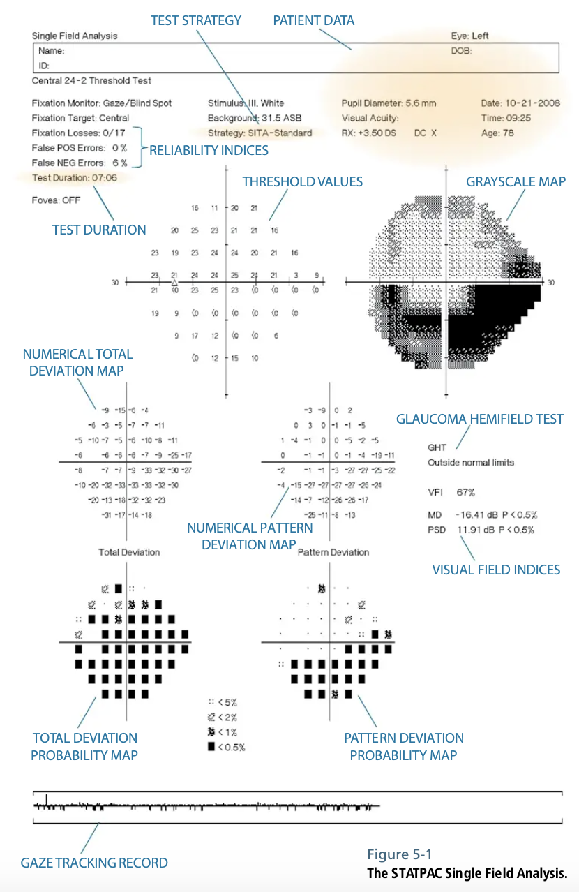
Figure 1. Image taken from Effective Perimetry (Zeiss Visual Field Primer, 4th Edition. Heijl, Bengtsson & Patella, 2012), Chapter 5: STATPAC Analysis of Single Fields, page 46.
Test Parameters
The top of the printout should contain the patient’s name and birthdate. Accuracy in birth information is key as the test results are compared to a normative database. Identify the trial lens power and ensure that the most appropriate prescription was worn during the test. The top parameters will also confirm what type of field test was performed; most often it is the 24-2 SITA threshold, but still confirm that the correct test was selected.

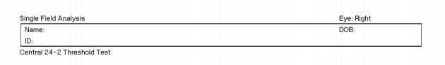

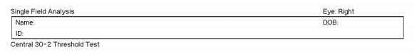
Figure 2 Top: Patient data for the Central 24-2 Threshold Test. Bottom: Patient data for the Central 30-2 Threshold Test.
Tip: Non-presbyopic patients should have their distance refraction inserted into the trial lens holder. Presbyopic patients should have their near refraction that is equivalent to a working distance of roughly 30cm (12”) placed into the trial lens holder, as the presented stimuli are closer than the standard 40cm (16”) working distance. You can estimate this to be +0.50 D more than their standard reading prescription.
Field Reliability

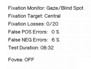
Figure 3: Field reliability. Image taken from Effective Perimetry (Zeiss Visual Field Primer, 4th Edition. Heijl, Bengtsson & Patella, 2012).
Fixation Losses
Fixation losses are measured by presenting a stimulus within the blind spot. If the patient responds to this stimulus, we can assume that the patient was not accurately looking at the fixation target. Fixation losses can also be continuously monitored by the gaze tracker. The ideal number of fixation losses should be less than 15-20% in order to deem the test as reliable. To avoid high fixation losses, have the technician properly align the patient and monitor their attention throughout the test.
False Positives
False positives occur when the patient responds, but no stimulus was presented. This is often referred to as a “trigger happy” patient. The higher number of false positives will give the appearance of a clearer visual field than expected. When these rates reach higher than 10-15%, the test becomes unreliable.
False Negatives
False negatives occur when the patient does not respond to a stimulus that they previously saw based upon earlier responses. This can often happen when a patient is “zoning out” or not paying attention during the test. Higher false negatives will give the appearance of more visual field defects than there actually are. When these rates reach higher than 10-15%, the test becomes unreliable.
Graphs and Plots
Gray Scale Plot

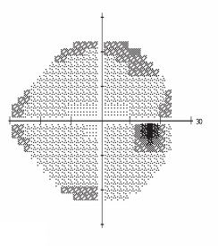
Figure 4: Greyscale plot. Image taken from Effective Perimetry (Zeiss Visual Field Primer, 4th Edition. Heijl, Bengtsson & Patella, 2012).
The grayscale plot provides a quick, general assessment of field defects. It does not go into full detail about the extent of each defect, therefore clinicians shouldn’t rely on this plot alone to identify field loss or progression. However, it is a great educational tool to show patients what their visual field appears to be and where their natural blind spot lies.
Total Deviation Plot
The total deviation plot demonstrates areas of one’s visual field that differ from the normative database in their age category. Each area of the visual field is represented twice; by the raw data in decibels (dB), and by shaded boxes. Clinicians should remember that the shaded boxes represent the probability that a test point is more likely to be abnormal compared to the surrounding points. Solid black squares have the highest probability of a true field defect compared to the lighter shaded squares.
Pattern Deviation Plot

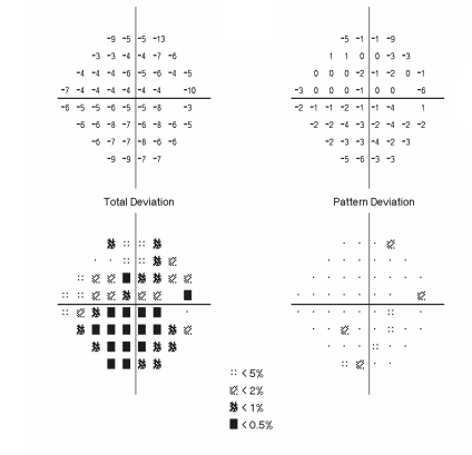
Figure 5: Total deviation versus pattern deviation. Top left: numerical total deviation map. Bottom left: total deviation probability map. Top right: numerical pattern deviation map. Bottom right: pattern deviation probability map. Image taken from Effective Perimetry (Zeiss Visual Field Primer, 4th Edition. Heijl, Bengtsson & Patella, 2012).
Total deviation plots are capable of outlining localized defects relating to glaucoma or visual pathway lesions; however, they can be masked by media opacities that cause larger, general depressions. This is where the pattern deviation plot comes in. Its job is to highlight localized defects associated with a disease or lesion after removing any suspicious generalized depression. The pattern deviation plot will do the best job in highlighting field defects that follow glaucomatous patterns. This plot also demonstrates areas of the visual field by raw decibels and by the shaded boxes of probability.
Global Indices

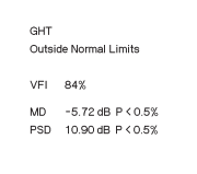
Figure 6: Global indices. Image taken from Effective Perimetry (Zeiss Visual Field Primer, 4th Edition. Heijl, Bengtsson & Patella, 2012).
Glaucoma Hemifield Test (GHT)
The glaucoma hemifield test was designed to detect glaucomatous visual field loss with high sensitivity and specificity and provides an easy-to-read analysis. It is not sensitive for retinal or neurological field loss. “Outside Normal Limits” or “Borderline” results indicate field loss that resembles glaucomatous defects. For clinicians who only occasionally interpret visual field tests, the GHT is the best marker to determine if a defect appears suspicious for glaucoma.
Visual Field Index (VFI)
One way to monitor progressive visual field loss is the visual field index. The VFI is more sensitive to changes in the central vision correlating with ganglion cell loss. The index represents the total amount of field loss in a percentage, with 100% meaning a completely normal field and 0% meaning perimetrically blind.
Mean Deviation (MD)
The mean deviation is a numerical representation of the total amount of field loss in decibels and is also used to monitor rate of change over time. Since the MD uses data from the total deviation plot, general depressions by media opacities can impact these results. Normal visual fields will range between 0dB to -2dB. When the MD becomes more negative, that indicates an overall decline in one’s visual field.
Pattern Standard Deviation (PSD)
Localized field loss is represented well by the pattern standard deviation. Lower PSD values close to zero indicate normal fields or generally depressed fields, while a higher value indicates moderate to advanced localized field loss. The PSD value is not as reliable for monitoring progression compared to MD and VFI.
In conclusion
When you get a Humphrey Visual Field report with shaded black spots, don’t get overwhelmed. Now that you understand the indices and markers on a field test, you will have a better understanding of the data presented before you to make the appropriate clinical decisions with confidence!
References
- Heijl A, Patella VM, & Bengtsson B. The Field Analyzer Primer: Effective Perimetry. 4th ed. Dublin, CA: Carl Zeiss Meditec; 2012.
- Chaglasian M. Sharpen Your Visual Field Interpretation Skills. Review of Optometry 2013. Retrieved from: https://www.reviewofoptometry.com/article/sharpen-your-visual-field-interpretation-skills


